Uncertainty-Aware Solar Forecasting
Developed probabilistic solar irradiance forecasting models using quantile regression and Bayesian neural networks, producing calibrated 95% prediction intervals from webcam imagery and meteorological data.
- ▸CNN-LSTM architecture processing paired webcam images and meteorological features for 2-hour-ahead GHI prediction
- ▸Quantile regression achieving 95.13% coverage with the sharpest prediction intervals (average certainty 0.7474)
- ▸Bayesian neural networks via BayesianTorch with Monte Carlo sampling for principled uncertainty estimation
- ▸Demonstrated that incorporating meteorological features significantly reduces interval width without sacrificing coverage
Overview
Short-term solar irradiance (GHI) forecasting is critical for grid stability and renewable energy integration, but point predictions aren't enough. Grid operators need to know how confident a forecast is. This project was done for EPFL's CFI Lab as part of the Machine Learning course (Professors Nicolas Flammarion and Martin Jaggi), introducing uncertainty quantification into GHI prediction and building on prior work by the Laboratory of Applied Photonics Devices (LAPD).
We investigated two complementary approaches, quantile regression and Bayesian neural networks, to produce calibrated 95% prediction intervals from webcam imagery captured on the EPFL campus.
Data
The project uses two complementary data sources collected on the EPFL campus:
- Webcam images captured from two distinct angles, providing visual perspectives of atmospheric conditions (resized to 224x224, normalized)
- Meteorological features: air temperature, cloud opacity, precipitable water, relative humidity, and solar zenith angle
For each image pair collected at a given time, the target is the GHI value 2 hours later. Data was split into training, validation, and test subsets.
Architecture
Both models share a CNN-LSTM backbone adapted from a deterministic baseline:
- CNN module: 4 convolutional layers (16, 16, 32, 32 channels) with 3x3 kernels, ReLU activation, batch normalization, max-pooling, and dropout (0.3 and 0.1)
- Meteorological MLP: 2 fully connected layers (32 neurons each, ReLU, dropout 0.1) processing the weather features
- LSTM: 2 stacked layers with 128 and 64 hidden units, combining image and meteorological features temporally
- Output head: Final MLP (64 neurons, ReLU) mapping to either 3 quantiles (QR) or a single value (BNN)
Training used Adam optimizer (lr=0.003), batch size 32, 200 epochs with early stopping (patience 30, min delta 0.3%).
Approaches
Quantile Regression directly predicts the 2.5%, 50%, and 97.5% quantiles using the pinball loss, which asymmetrically penalizes under- and over-predictions at each quantile. A non-negativity constraint is applied only at inference (not during training) to keep GHI physically realistic while allowing the model to learn freely.
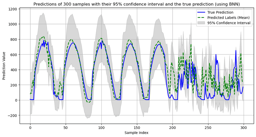
Bayesian Neural Networks replace deterministic weight layers with probabilistic equivalents (via the IntelLabs BayesianTorch library), treating weights as distributions. During inference, 50 Monte Carlo forward passes produce a distribution of outputs: the mean gives the prediction, and the standard deviation gives the uncertainty. Training minimizes a combined data loss + KL divergence term to regularize the posterior.
Results
We evaluated on three metrics: percentage of true values within the predicted bounds, average certainty (inverse of interval width, i.e. interval sharpness), and MSE. The best configuration, quantile regression with meteorological inputs, reached:
95.13%
Empirical coverage
0.0214
MSE
0.7474
Interval certainty
2 h
Forecast horizon
Full comparison across configurations:
| Model | Within Bounds | Avg Certainty | MSE |
|---|---|---|---|
| QR + Meteo | 95.13% | 0.7474 | 0.0214 |
| QR (images only) | 94.93% | 0.6533 | 0.0329 |
| BNN + Meteo | 92.22% | 0.6624 | 0.0244 |
| BNN (images only) | 96.55% | 0.5432 | 0.0200 |
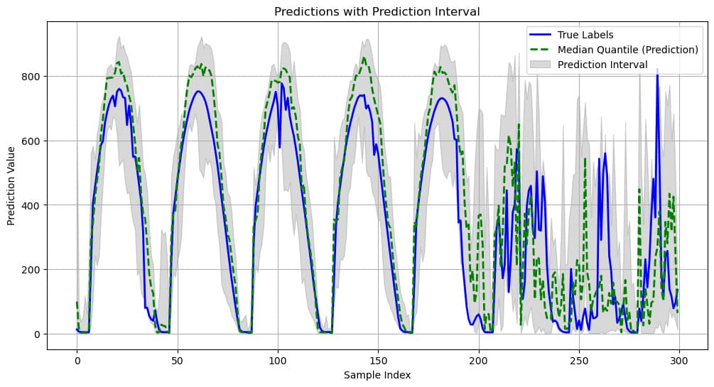
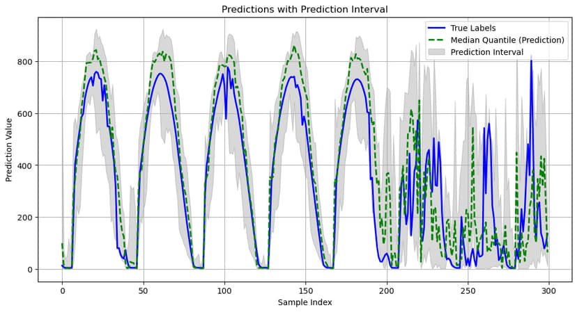
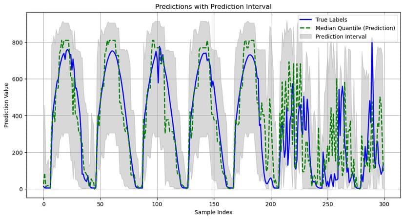
The comparison below shows the effect of meteorological data on quantile regression. Without it, intervals are noticeably wider and median predictions deviate more from true values:
Key findings:
- Quantile regression with meteorological data produced the best balance: 95.13% coverage with the sharpest intervals (highest certainty) and low MSE
- Meteorological features significantly improved interval sharpness without sacrificing coverage
- BNNs tended to over-estimate uncertainty with wider intervals; the images-only BNN reaches the highest coverage (96.55%) but the lowest certainty (0.5432), since over-wide intervals inflate coverage, likely from weight over-regularization
- Preliminary experiments with a pretrained ResNet18 backbone showed promise (certainty 0.8197, MSE 0.0223 after only 14 epochs)
What I Learned
- The distinction between aleatoric and epistemic uncertainty isn't just theoretical; it directly determines which modeling approach works better
- Quantile regression is surprisingly effective for well-calibrated intervals with minimal computational overhead compared to full Bayesian approaches
- Calibration and sharpness are in tension: BNNs can easily achieve high coverage by producing very wide intervals, but that's not useful operationally
- Webcam imagery contains meaningful signal for solar forecasting: shadows, reflections, and sky conditions encode information that meteorological sensors miss